The concepting and implementation process of the Vis2 CNN project

Motivation

While spending time to study neural networks mainly last summer, often I was faced with the difficulty of being able to understand how convolutional layers are connected with each other, but also to different types of layers. When a fully connected layer is connected to another fully connected layer or to an output layer, it is quite simple to understand that for each possible pair of nodes there exists one weighted edge. With convolutional layers the situation is a bit different, as weights are shared among several neighbourhoods of nodes, but also because there more dimensions to deal with: In a fully connected layer, the shape of the weight matrix is two dimensional [n_input, n_output], while a convolutional layer has a four dimensional shape of [kernelwidth, kernelheight, inputdepth, outputdepth].

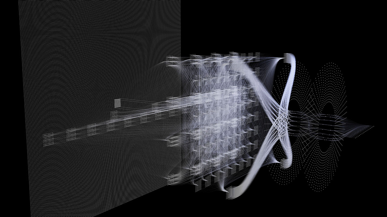
This four dimensional connectivity allows for unusual calculations such as a 1x1 convolution, which sounds absurd to a person used to dealing with image processing, but is perfectly valid in the four dimensional connectivity of a convolutional layer: We just connect each input pixel to the pixel at the same 2 dimensional position in all of the output feature maps, thereby creating a set of fully connected layers each dedicated to a spacial location. When teaching such concepts, it is not easy to confuse the listener, especially without a clear visual representation. Although there exist a number of different types of schematic views, most are too simplified and focus only on certain aspects of the layers, that allow a broad overview of the architecture but are still unintuitive for beginners.

My goal was therefore, to make a tool that allows someone trying to explain CNNs to interactively expand and reduce, reshape, recombine etc… a number of CNN components in full 3D, to be able to show the different aspects of a CNN with good visual representation.

The concepting phase

I started building a prototype of the visualization in the 3d Software Houdini, as it provides a good environment to sketch out ideas based on procedural geometry with a good balance between preexisting components and full access to geometry manipulation with the embedded vectorized C-Similar language VEX. I thought a lot about which interactive controls and which levels of detail I should implement and developed the main concepts, such as expanding the weights to show all convolutional calculations, arranging the featuremaps in different axes or shapes, edge bundling, etc. in Houdini. It was very important to have a clear plan of what to implement for the real time version in Unity, as I had to generate 100% of the geometry in code without being able to use pre-existing components. This concepting phase was already completed by 90% before giving the first presentation, afterwards, if I remember correctly, I only got inspired by a colleagues presentation to include edge bundling, which was not on my list before.

Bird

The node editor in Houdini. The visual programming of constructing a graph of interconnected geometric operations allows for a quick prototyping process when designing a new visualization type, as all the parameters can quickly be accessed on the respective node.

Bird

Implementation

As I was a complete beginner at using Unity before starting the implementation of this project, first I had to figure out a lot about the possibilities of the engine, mainly regarding customization of shaders and procedural geometry. As a game engine, Unity is mainly made for video games, and its very strong portability makes some compromises in customization. Shader varyings for example are not possible in Unity’s own language Shaderlab, only variables with predefined semantics can be passed between the vertex, geometry, and fragment stage. Also there is no way to arbitrarily assign vertex attributes, only the predefined ones like position, color, uv, etc., so writing a custom shader can be quite a restricted experience.

I also researched a lot about instancing, because my initial plan for the line rendering was to have one curved line that is instanced with distinct transformations for each required graph edge, but after some experimenting and after I found this article dealing with instancing vs. two shader based methods, I decided to go with a geometry shader based method for generating the lines. Shortly explained, the start and end points are passed to the vertex shader and directly forwarded to the geometry shader, where based on the 3d positions of the start and end points, an adjustable number (max 20) of curve points are interpolated, using a logistic curve with adjustable scale as curve interpolator. They are then transformed into clip space, where a test for negative values of the homogenous component w is done to discard any vertices that are behind the camera. This is necessary as doing the MVP transformation in the geometry shader skips the automatic clipping stage between vertex and geometry shader. Based on the curve points that now are represented in clip space, the normals for each curve sections are calculated and used to add 2 vertices in either direction to give the line some width. The line width is a blend between an absolute value and a perspective width that decreases by distance, with a user adjustable bias between the two. All in all, the lines can consist of a maximum of 120 vertices, which is an already quite high number and restricts the usage of per vertex variables as the maximum (allowed by Unity) scalar float equivalent number of variables created in the geometry shader is 1024.

In the fragment shader, the color and alpha lookup is done based on the distance to the center, and also based on a red/blue color map to visualize both positive and negative values in when actual weight values are set. The shader for the pixel/node shapes is quite similar, but only generating 2 triangles forming a square for input points in the geometry shader and allowing the rendering of either the full square or a circular shape with a brightness falloff towards the edge to simulate a shaded sphere. The transperency of the node sprites causes some z order issues where pixels behind can be discarded in the depth test, but I found this not to be a big issue as the nodes are quite small in the frame anyway usually so I didn’t go ahead with initial intentions of rewriting the shader to construct a more detailed circular triangle fan instead of just a square.

Bird
Bird

Generating the geometry

The geometry is calculated 100% procedurally in code, so a number of Shape generator classes had to be written and then combined to be able to calculate the highly variable and interdependent meshes for the various layers. Major challenges I faced were the adaptive optimization when certain complexity reduction parameters were fully enabled, like for example the seamless expansion of showing only the filters to showing all calculations or edge bundling, where a quadratic number of edges suddenly gets reduced to a linear number of edges (regarding point number) when they merge in the center. As the parameters are all seamlessly interpolated to allow for smooth interactive parameter changes, many special geometric combinations had to be thought of and implemented.

Loading the Tensorflow Checkpoints

This was a challenge on its own, as the Tensorflow-native .ckpt format, which stores the necessary data to reconstruct a model graph and read the weight and activation values is binary and requires careful name/”collection” assignment during the construction of the model for querying specific layers afterward by name/”collection”. Also activation values of the layer units (activations are taken from the ReLU-Layer that is appended to each of the convolutional layers) are not stored in the file, but have to be queried by running a test sample through the restored restored graph. For being able to show the development, I’ve written out checkpoint files for a simple CNN trained on the Cifar10-greyscale dataset (classification between 10 classes by 32x32 images) after each of 10 training epochs (epoch = training iteration over all training samples), as well as the untrained, randomly initialized weights at the beginning. The converter program then loads each of those checkpoint files, starts a tensorflow session, and feeds a training example as into the graph to be able to query the activation values of each layer. Then a json file is written that stores the name, shape, weight and activation values for each layer. This json file is about 10 mb per epoch per test sample, which leads to relatively long loading times when switching test sample in the program. This could be optimized by either reducing the float value precision in the json or serializing the data into a Csharp readable format once it has been read from the json. The weight values are then used to assign color data to the Unity Mesh of the respective layer.

Demonstration of functionality / parameters

Scrubbing through the epochs, displaying the layer weights over the course of the training.

Scrubbing through the epochs, displaying the early conv layer activations over the course of the training.

Scrubbing through the epochs, displaying the later conv layer activations over the course of the training.

Transition to the mode where all inference calculations are shown as edges.

Transition of a convolutional layer to the edge-bundled visualization.

Switching the featuremap layout between linear and grid.

Different layout shapes of the fully connected layer.

Collapsing the feature map outputs of a convolutional layer for simplicity, as these are usually quite numerous.

Edge bundling of fully conntected layers. This can be quite useful to show a large number of units in fully connected layers while still keeping visual simplicity and performance adequate.