User Guide
Sliceview Interface
After startup the application provides the user with the sliceview interface and the transferfunction window disabled. The first step will be to load a dataset, which is simply done by clicking on File -> Open. In the file dialog, it is possible to choose bettween files of 2 formats: .dat and .gdat. Gdat(Gradient - dat) is the applications own format which also contains precomputed gradients and histograms for 1D and 2D transferfunctions.
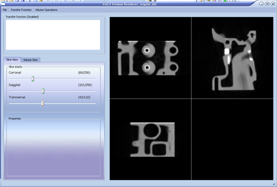
After the Volume is loaded, the user is now able to slice through the volume with the sliders provides in the sliceview interface. The main window is parted into the 3 main slice axes. When the user doubleclicks into one of the main axe subwindows, then this window is maximized.
1D Transferfunction
In order to provide a better insight into the volume, the user is now able to load a 1D transferfunction via the Transfer Function -> Load menu. This dialog supports .btf (binary transfer function) and .bt2f (binary transfer 2 function) files. In case of the sliceview interface, only the 1D version will be applied to the slices.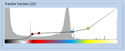
Another possibility is to create a new transferfunction, which is simply done by enabling the 1D Transferfunction via Transfer Function -> Mode -> TF 1D. Then the user is able to add points in the transferfunction window by clicking, drag the points by click and drag, remove points by right doubleclick, do a windowed zoom of the histogram by middleclick and drag or zoom the whole window by ALT + doubleclick. When the result is satisfying the transferfunction can be saved in the Transfer Function menu.
The changes of the transferfunction are reflected immediately by the sliceview window. The current image of the main window can be saved with File -> Save Image
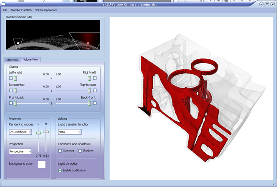
Volumeview Interface
The user is able to change from the sliceview interface into the volumeview interface by changing the tab. There the user is provided with certain rendermodes (the latter 2 will be described seperately):
- MIP - Maximum Intensity Projection
- DVR FTB
- DVR BTF
- DVR Combined
- Curvature
The user now sees a 3D version of the dataset loaded before in the main window, and is also able to interact with it in the following way:
- Rotate around the dataset: left click + drag
- Zoom in/out of the dataset: right click + drag
- Pan through the dataset: middle click + drag
- Reset view: right double click
The Projection can be changed in the Projection drop down menu between perspecive and orthogonal. Because perspecitve projection is the more natural way of seeing things, it is chosen by default.
2D Transferfunction
The 2D transferfunction can be enabled in two ways, first it is possible to load a 2D transferfunction from disc or by enabling it via Transfer Function -> Mode -> TF 2D. Then the user is now able to place Triangles with differend colors in the Histogram.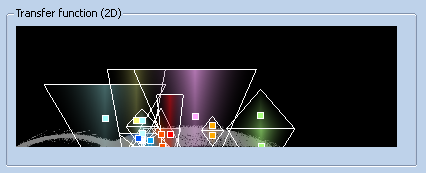
The user cann zoom in into the histogram with ALT+left doubleclick. The Triangles can be dragged like in the 1D version, scaled with CTRL+ click + drag. The scale with respect to the width of the triangles is restricted, hovewer, the height can be scaled also by a negative factor. This way, the user can mirror the triangle horizontally. Other possible shape adjustment is skewing done by pressing CTRL+drag and drop. The changes in the transferfunction are reflected in realtime in the volumeview.
Combined DVR Mode
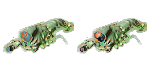
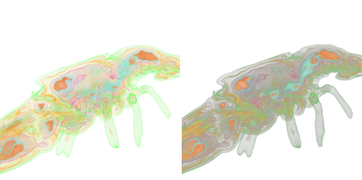
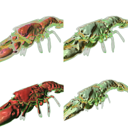
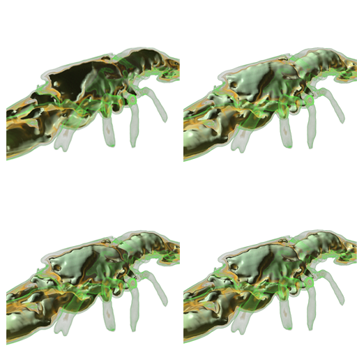
The combined mode combines regular DVR rendering with shading an Isosurface with a certain illumination model. The Illumination Models the application provides are Phong - Blinn, Toon, Metal. When the combined is chosen, two additional sliders appear in the gui, which are for choosing the high and low threshold (see the image below for different thresholds, and the comparison to orthographic projecton in the lower right) of the density where the voxels should be shaded. In this case it is now possible to rotate the lightsource around the volume by clicking on Enable Modification in the Light Direction section. Then the user is able to rotate the lightsource by clicking and dragging in the volumeview window.
In order to improve the visual quality of the shaded images contours and shadows can be added to the created images simply by enabling the appropriate checkboxes.
Both are updated in realtime when the camera is rotated around the volume or the lightsource is moved. The same can be done when Toon or Metal shading is used.
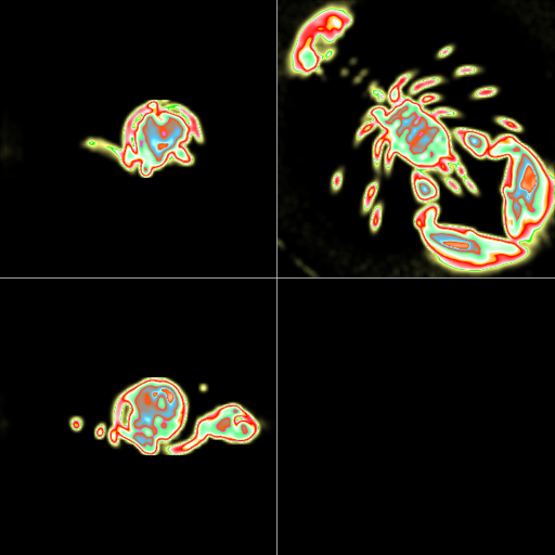
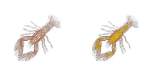
Curvature Mode
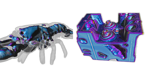
It is also possible to visualize the curvature of the surface defined by first hit of the voxel with density between the specified tresholds.
Clipping Planes
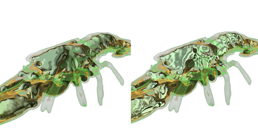
It is possible to clip the volume at the three main axis in both positive and negative directions, in order to get an insight into the volume with preserving the contextual information from the region around. This can be done by simply enabling the checkboxes and moving the appropriate slider. The image below shows a comparison between clipped volumes with differen lower boundaries (during phong shading). In the image on the right it is possible to see the composited inside whereas on the left, everything inside is solid.